Exploring the Basic Concepts and Strategy of Market Volatility
In this article, we examine volatility and the unique opportunities it presents for traders. Volatility typically describes the extent of price fluctuations in relation to an asset’s average value. The most prominent measure of volatility is standard deviation; however, several other tools such as Average True Range (ATR) and Bollinger Bands are commonly used in trading system development.
All these tools share a common feature: they measure historical volatility, evaluating how an asset’s price has changed over a set period.
Defining Implied Volatility
Introducing new concepts can deepen understanding, and here we present implied volatility. Unlike historical volatility, which considers past prices, implied volatility forecasts an asset’s future price movements. This measure reflects the market’s expectations regarding the asset’s volatility going forward.
Implied volatility is derived from the prices of complex financial instruments like options on the S&P 500, one of the most significant market indices. It is quantified through the VIX Index, often referred to as the “Fear Index.” This nickname arises from its inverse relationship with the Stock market; the VIX typically rises during anticipated market downturns and volatility, while it declines during stable periods.

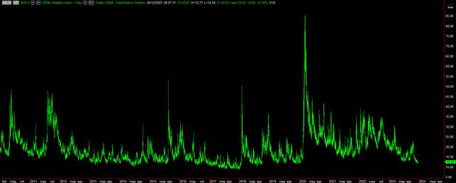
Figure 1 illustrates the historical trends of the VIX Index ($VIX.X) from 2010 to the present.
The VIX Index demonstrates unique behavior: it remains relatively stable, fluctuating around average values, but shows sharp, significant spikes during market crashes.
Broadly, there are two primary methods for capitalizing on market volatility. The first method employs implied volatility, like the VIX Index, as a tool for trading decisions. This is parallel to using historical volatility tools such as standard deviation, average true range, or Bollinger Bands. This approach aims to restrict trading activity, particularly in equity futures, concentrating on trades with higher success probabilities.
The second method, which we will explore in this article, focuses on creating a trading strategy specifically aimed at implied volatility, involving instruments that replicate implied volatility.
Trading Strategy for VIX Futures (@VX)
This strategy deals with VIX Futures (@VX), which are traded on the CBOE in Chicago, using the VIX Index as the underlying asset.
As noted earlier, the VIX Index exhibits strong mean-reverting characteristics. To evaluate this property, we created a simple trading system based on Bollinger Bands, analyzing it with a 30-minute chart. Our backtesting period spanned from January 2010 to November 2023 during standard trading hours (5:00 PM to 4:00 PM).
The trading strategy entails entering a short position when the price falls below the upper Bollinger Band (“UpperBand”), and entering a long position when the price breaches the lower Bollinger Band (“LowerBand”). A risk management strategy with an initial stop loss of $2,000 is implemented.
Here is the EasyLanguage code for our strategy:
inputs: MyStop(2000);
inputs: Length(20), NumDevs(2);
variables: UpperBand(0), LowerBand(0);
UpperBand = BollingerBand(c, Length, +NumDevs);
LowerBand = BollingerBand(c, Length, –NumDevs);
if C crosses under UpperBand then Sellshort next bar at market;
if C crosses over LowerBand then Buy next bar at market;
if MyStop > 0 then setstoploss(MyStop);
setstopcontract;
Figures 2 and 3 display examples of trades along with the backtesting results.

Figure 2 shows an example of a short trade executed using the Bollinger Bands trading system on VIX Futures.

Figure 3 presents the Strategy Performance Summary for the Bollinger Bands trading system on VIX Futures.
Reviewing the results indicates that the strategy works effectively primarily on the short side. To understand this discrepancy better, let’s review Figure 4, which illustrates long-term trends of the VIX Index and VIX Futures.
Figure 4 compares the VIX Index (@VIX.X) and VIX Futures (@VX).
The correlation between the two indices is evident; every spike in the VIX Index is mirrored by a spike in VIX Futures, though the intensity may differ. Notably, a significant devaluation in VIX Futures over time is apparent. What accounts for this pattern?
The explanation lies in futures pricing. VIX Futures typically trade at a premium over the index. In the absence of market anomalies or crashes, this premium diminishes daily, converging with the index value upon expiration.
This means a long-term downside bias exists, rendering the mean-reverting approach ineffective on the long side of the strategy.
Refining a Volatility Futures Trading Strategy Focused on Short Selling
Our next step is clear: we will refine our trading strategy by placing a stronger emphasis on short selling.
Optimizing a Mean-Reverting Strategy for Volatility Futures (@VX)
Initially, we evaluated whether the standard Bollinger Bands settings—20-bar length and 2-standard deviation—were indeed optimal for VIX Futures. To find better parameters, we adjusted the settings by varying the “Length” from 10 to 30 bars in increments of 5 and the “NumDevs” (number of standard deviations) from 1 to 3 periods in increments of 0.5. Additionally, to mitigate weekend overnight risks, we implemented a policy to close all positions by Friday evening.

Figure 5. Optimization results for the “Bollinger Bands short only” trading system on VIX Futures.
The optimization results indicated that decreasing the Bollinger Bands length from 20 bars to 15, while maintaining the standard deviation at 2, led to better performance. As a result, net profit rose from $145,220 to $158,350, and the average trade value improved from $160.82 to $172.60. We have decided to adopt these new parameters.
Figure 6. Detailed Equity Curve of the “Bollinger Bands short only” trading system on VIX Futures.
Previously, we assumed a full trading session from 5:00 PM to 4:00 PM for our operations. To enhance results, we will explore if restricting this time window could yield superior outcomes. Furthermore, we will analyze the optimal duration for which a position should remain open, adhering to our existing rule of closing all trades by Friday afternoon.
Utilizing a proprietary function, we integrated these time constraints into the system’s code and performed an additional parameter optimization.
Figure 7. Time window optimization for the “Bollinger Bands short only” trading system on VIX Futures.
Figure 8. MaxDaysInTrade optimization for the “Bollinger Bands short only” trading system on VIX Futures.
The optimization process for the time window indicated that the most profitable hours of operation are not the full 23-hour span (5:00 PM–4:00 PM) but rather a narrower range from 6:00 PM to 2:00 PM. Additionally, the analysis determined that a maximum trade holding duration of five days is most effective. Exceeding this period does not yield significant benefits and actually elevates market risk exposure.

Figure 9. Strategy Performance Summary and Total Trade Analysis after optimizing the time window and MaxDaysInTrade.
At this stage, our analysis has begun to yield initial conclusions regarding the trading system. Positive metrics indicate improvements in both net profit and average trade value. However, it is critical to note that the current average trade remains insufficient for the instrument in question. The @VX Future carries a tick value of $50, necessitating an average trade size of at least $250-$300 for live trading. Moreover, the maximum drawdown is still considerable, exceeding $40,000. While this reflects the market volatility triggered by the COVID-19 pandemic in 2020, further enhancement is necessary to prepare for future cyclical market corrections.
How can we further enhance our trading system?
One strategy could be to evaluate specific price patterns. We will utilize a proprietary list of scenarios to optimize the system for identifying the best-performing pattern. Through this optimization process, Pattern 39 emerged as a significant option, notably reducing drawdown from $44,160 to $23,970, albeit at the cost of some net profit. The criteria for Pattern 39 stipulate that the difference between today’s high and open must be smaller than the difference between yesterday’s high and open. This pattern implies market uncertainty and compression, suggesting a forthcoming defined direction, specifically a downward trend.

Figure 10. Optimization of the price patterns in the “Bollinger Bands short-only” trading system on VIX Futures.
As a final improvement, we might implement a Breakeven Stop. This stop activates when an open position reaches a defined profit threshold, effectively safeguarding a winning trade from reverting to a loss. Although such a stop might not always boost overall strategy performance, it offers a sense of security for traders, particularly in today’s market environment. We will test this method concurrently with optimizing the initial stop.
Effective Trading Strategies for VIX Futures Revealed
In recent analysis, a method known as the “Bollinger Bands short-only” trading system was examined for its efficacy on VIX Futures. This study highlights critical optimization efforts for stop loss and breakeven points tailored to improve trading outcomes.
Figure 11 illustrates the optimization of stop loss and breakeven stop orders within this trading framework.
Figure 12 presents a detailed equity curve reflecting performance after optimizing the trading strategy.

Figure 13 summarizes the strategy’s performance, showcasing total trade analysis post-optimization.
Key Takeaways: Effective Mean-Reverting Trading on VIX Futures
In conclusion, the refined trading strategy has demonstrated substantial success, securing a net profit of $173,300 and an average trade yield of over $240. This evidence suggests a reliable baseline for establishing a live trading system for VIX Futures (@VX). The mean-reverting approach has emerged as a productive method for navigating volatility within futures trading.
This strategy is adaptable for other instruments, including ETFs or CFDs that track VIX performance—though minor modifications may be necessary to tailor its effectiveness. Traders are encouraged to continue exploring this strategy, testing its application, and refining it for enhanced performance.
As we venture further into the trading landscape, ongoing experimentation and learning remain essential. This strategy provides a robust launchpad for those seeking to improve their trading practices.
Wishing you successful trading experiences!
Andrea Unger